Cigarette Consumption — Cigar • phtt

a panel of N=46 observations each with time-dimension T=30 from 1963 to 1992

total number of observations : 1380

observation : regional

country : United States

Usage

data(Cigar)

Format

A data frame containing :

state: state abbreviation
year: the year
price: price per pack of cigarettes
pop: population
pop16: population above the age of 16
cpi: consumer price index (1983=100)
ndi: per capita disposable income
sales: cigarette sales in packs per capita
pimin: minimum price in adjoining states per pack of cigarettes

Source

Online complements to Baltagi (2001). http://www.wiley.com/legacy/wileychi/baltagi/.

References

Baltagi, Badi H. (2001) Econometric Analysis of Panel Data, 2nd ed., John Wiley and Sons.
Baltagi, B.H. and D. Levin (1992) “Cigarette taxation: Raising revenues and reducing consumption”, Structural Changes and Economic Dynamics, 3, 321--335.
Baltagi, B.H., J.M. Griffin and W. Xiong (2000) “To pool or not to pool: Homogeneous versus heterogeneous estimators applied to cigarette demand”, Review of Economics and Statistics, 82, 117--126.

Examples

data(Cigar)
## Panel-Dimensions:
N <- 46
T <- 30

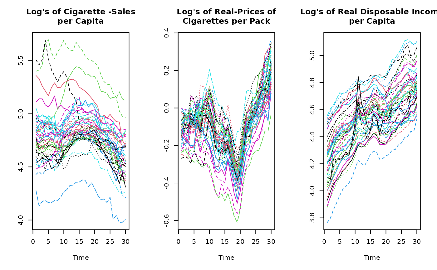
## Dependent variable:

  ## Cigarette-Sales per Capita
  l.Consumption    <- log(matrix(Cigar$sales, T,N))

## Independent variables:

  ## Consumer Price Index
  cpi        <- matrix(Cigar$cpi, T,N)

  ## Real Price per Pack of Cigarettes 
  l.Price    <- log(matrix(Cigar$price, T,N)/cpi)

  ## Real Disposable Income per Capita  
  l.Income   <- log(matrix(Cigar$ndi,   T,N)/cpi)


####################
## Plot the data  ##
####################

par(mfrow=c(1,3))
## Dependent variable
matplot(l.Consumption, main="Log's of Cigarette -Sales\nper Capita",
        type="l", xlab="Time", ylab="")
## Independent variables
matplot(l.Price, main="Log's of Real-Prices of\nCigarettes per Pack",
        type="l", xlab="Time", ylab="")
matplot(l.Income, main="Log's of Real Disposable Income\nper Capita",
        type="l", xlab="Time", ylab="")

par(mfrow=c(1,1))